Everything I need to know about causality, I learned smoking cigarettes
I've gone through a causal inference revolution, and I can't go back. Causal inference is all I think about now, but unfortunately its importance is often overlooked. Part of my revolution came after reading Miguel Hernán et al's paper on infant mortality and smoking, The Birth Weight "Paradox" Uncovered?. It took me a full evening to really understand its points, and it was rewarding when I finally did. In this blog post, I'm going to examine the paper from my point of view, and add or expand on details that I wish the original authors had. In writing this blog post, I have two goals in mind. The first is to solidify the ideas in my head. No better way to do that than to have to explain it to others. The second goal is to provide a shortcut for others to understand why causal inference is important.
Introduction
The authors start by saying that researchers will naively stratify a risk factor, like smoking, by the birthweight (BW) of infants. Researchers noticed that if the risk factor produced low birthweight (LBW) infant more often, then there would be a specific birthweight where infants below this threshold would have a lower mortality if in the riskier group. For example, for infants born below ~2000g, those infants who were exposed to maternal smoking actually had a lower infant mortality rate than those not exposed to maternal smoking. See figure below:
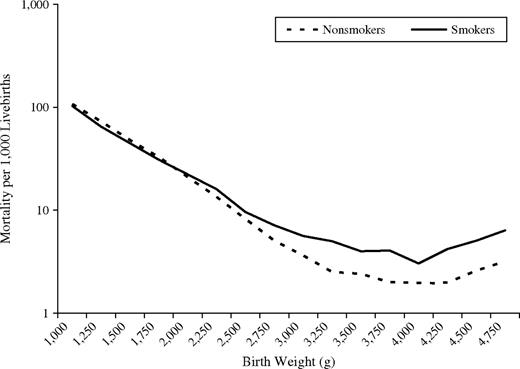
This seems like madness - not smoking is associated with higher infant mortality in some populations! Some researchers have even suggested that:
"the effect of maternal smoking is modified by birth weight in such a way that smoking is beneficial for LBW babies."
Let's investigate what is really going on.
Material and Methods
The authors use a large dataset of over 3 million infants. They define LBW as less than 2500g. Their metric of interest, infant mortality, is defined as a death in the first year per 100,000 livebirths. How do they summarise the effect of maternal smoking?
"We used logistic regression to estimate infant mortality rate ratios and 95 percent confidence intervals..."
In other words, they will be using a specific coefficient in a logistic regression model to produce a summary of the effect of maternal smoking on mortality. Specifically, if we let \(M\) denote the presence of maternal smoking (0 or 1) our model might look like:
$$\text{logit}(p_i) = \beta_0 + \beta_1 M_i $$
and so \(\beta_1\) summarizes the effect of maternal smoking. We'll call the above model the "crude" model. Let \(B\) denote birthweight. We call the following model the "adjusted" model:
$$\text{logit}(p_i) = \beta_0 + \beta_1 M_i + \beta_2 B_i$$
The next question to ask is what else to control for in this regression. The authors say:
"control for potential confounders (maternal age, gravidity, education, marital status, race/ethnicity, and prenatal care). Since adjustment for these potential confounders had virtually no effect, we present only the unadjusted rate ratios below."
What does this mean? If we extended the model to:
$$\text{logit}(p_i) = \beta_0 + \beta_1 M_i + \beta_2 B_i + \beta \cdot C_i$$
where \(C\) are other controls mentioned above, this doesn't change the conclusion (or the coefficients - it's not clear), so the author choose to present results without the additional controls.
Naive Analysis Results
After running the regression, the crude model produced that \(\beta_1 = 0.438 \pm 0.029 \). (The paper actually uses the rate ratio, which is the exponential of the coefficient in the model - we won't). However, if we use the adjusted model, then \(\beta_1 = 0.049 \pm 0.032 \), a 10-fold decrease. What happened? Why, after conditioning on BW, did we seem to lose so much effect? It gets worse, in fact.
If we stratify the population into LBW and non-LBW (a "stricter" way to control for a continuous variable), and train the crude model on both these sub-group, we see that smoking actually benefits the infants in the LBW sub-group: the rate ratio of maternal smoking less than 1 (the opposite conclusion is found for the non-LBW sub-group).
Possible causal diagrams
I'm going to assume the reader is familiar with causal diagrams. I really liked that the authors went through increasingly complex causal diagrams to explain the paradox. I'll do the same. (Diagrams produced by my latest side project, dog).
Diagram 1

This is the simplest model of our causal relationships. Smoking causes LBW, but has no direct effect on mortality, except through LBW. A very useful thing I learned from this paper is that a causal diagram has implications that the data should support, and if the data doesn't support it, the causal diagram is invalidated! Let's see how this works using the results from the regressions. If the above causal diagram is true, then smoking and mortality are certainly correlated. And we see this in the crude regression above (the coefficient is not 0). On the other hand, this diagram also implies that conditioning on BW means that smoking and mortality are independent. However, in the adjusted model above, where we do condition for BW, we still see that the coefficient of smoking is still far from 0. Thus, the data suggests that smoking and mortality are dependent, conditioned on BW. Hence, this diagram is wrong.
Diagram 2

We had success with our implication test above. Let's try the same test on this new causal diagram. In the above causal diagram, if we condition on smoking, LBW and mortality should be independent. However, in the adjusted model, LBW has a non-zero coefficient. So we can refute the above diagram.
Diagram 3

In this new model, we have smoking causes LBW, smoking causes mortality and there is a causal relationship between LBW and mortality. We see that LBW is a mediator for smoking. The authors are more precise and say that smoking is partially mediated through LBW, since there still is a direct effect of smoking on mortality. The authors state that this DAG is actually the simplest model, because it is "complete" (I suppose they mean this in the graph-theory sense of "complete"). In other words, the previous two graphs had very strict constraints on relationships that allowed us to "test" the graphs. The above graph doesn't have this property, and technically has the least amount structure. However, it probably presents the most accurate model of reality thus far.
This is where the story gets interesting. If you showed this model to domain experts, they would say it is too simple. A domain expert would suggest that there are other, possibly unobserved, factors involved in BW, like birth defect. If this is true, bad things can happen. Let's explore this in diagram 4. (From here, I'll actually diverge a bit from the paper, but only because the paper does it's presentation of diagrams in an odd manner.)
Diagram 4

This new diagram introduces an unobserved variable (in blue), birth defects, and removes some causal links - but as we'll see even this simple diagram is enough to give us our "paradox". Birth defects also causes LBW and also has a (strong) positive effect on mortality. So, given this diagram, let's see what happens when we condition on LBW. Among LBW infants, if the mother didn't smoke, then we know the only other cause for LBW was birth defects. By conditioning on LBW, we have introduced a spurious correlation between smoking and birth defects ("if not this, than that") - in fact, this association is negative. And because birth defects has a positive association with mortality (and smoking has none), we have introduced a negative association between smoking and mortality.
The problem occurs because birth defects is unobserved. If we had observed birth defects, we could have controlled for it and everything would have been fine.
The story above doesn't mention observations - so why is observation so important? Even though we don't observe birth defects, the "effect" of it is still present in the outcomes. And because BW is caused by it, the effect of birth defects is passed through to BW in any analysis. This means that even though BW has no effect on the outcome, it will still look like it because it's highly correlated with birth defects.
Diagram 5

Let's introduce a link between smoking and mortality now. The authors state
In this case, the rate ratio adjusted for birth weight would be a combination of 1) the true direct effect of smoking on mortality and 2) the bias resulting from the presence of common causes of LBW and mortality.
It's not obvious which effect is larger in magnitude, apriori. Similar to above, if we could control for birth defects, this bias would vanish.
Diagram 6

With this diagram, we've added a link between LBW and mortality, adding more plausibility to our diagram. The same bias still remains, however.
Diagram 7

The authors then put forward another diagram that suggests that only some types of low birth weight (LBW_B) are actually harmful. The argument is as follows.
Some instances of LBW are not harmful, like being born in a higher altitude. That is, LBW caused by higher altitude infants do not see a higher risk than their counterfactual counterparts born at normal BW in a low altitude area. This LBW is of the type LBW_A. However, a LBW in a low altitude area is of much higher risk, since the cause of the their LBW isn't LBW_A but LBW_B, and is of much higher risk. In this case, if we condition on LBW, we would introduce the same biases observed above.
Discussion
This is probably my favourite part of the paper. The authors ask "why are we conditioning on BW anyways?" Researchers can be interested in two questions: what is the total effect of smoking, and what is the direct effect of smoking (aside: I learned a lot about the differences between total and direct effects by reading about the Table 2 fallacy.) If the researchers' goal is compute the total effect of smoking on mortality, then adjustment for a child variable (like BW) is not correct. (The author's state that, for many sensible reasons, BW is a cause of smoking, and not vice versa). In fact, the only adjustment needed is for confounders of smoking and mortality. This, according to the back-door criteria, is sufficient to compute the total adjustment.
However, if the researchers goal is to compute the direct effect, things are more difficult. To compute a direct effect, one needs to control for any mediators of smoking. This makes controlling for BW sensible. But then, we need to make sure that if those mediators are colliders (have more than a single cause), we need to control for all their parents too to satisfy the backdoor criteria. This is what happened in Diagram 4 above: because we conditioned on BW, but failed to condition on unobserved birth defects, our estimate of the direct effect of smoking was biased.
In reality, I imagine the original researchers did not have a causal diagram in mind when they first encountered the paradox. I doubt they even had the vocabulary of direct or total effects.
In conclusion, I hope this articled helped understand this highly important and influential paper. Apriori, we know that smoking is bad (hence the confusing "paradox"), but how often might this happen in less conspicuous contexts? Without explicitly drawing or stating a causal diagram, it's easy to make the researchers' original mistake and think some interesting phenomenon is occurring.